Why an Off-Grid Telecom Solar Simulation Can Give a False Pass

A telecom solar simulation gives a false pass when it counts energy that the proposed system cannot store. In a hypothetical design, a charging path limited to 1 kW cannot accept 5 kW of surplus photovoltaic (PV) power. Omitting that constraint produces an optimistic battery trace for a system the proposal does not contain.

An hourly energy balance must follow production, live demand and accepted charging on the same clock. A daily solar total can look sufficient while storage runs down between production periods. This review checks that particular model error; the wider process from load survey to commissioning remains in the Telecom Site Energy Guide.

Can the battery accept the charging power shown by the simulation?

The battery can accept the simulated charging power only when the conversion path can deliver it within the applicable battery charge limits. Available PV surplus is a charging opportunity, not energy already stored. The model must also respect battery headroom and applicable voltage, temperature and battery management system (BMS) restrictions.

Consider one hour with 6 kW of potential PV output at the protected direct current (DC) bus and a simultaneous 1 kW load. PV serves the load first, leaving 5 kW. If charging is limited to 1 kW at that bus, at most 1 kWh enters the charging path during the hour. With an assumed 90% charging efficiency, storage gains 0.9 kWh; the remaining 4 kWh of potential PV is curtailed.

Remove the power limit and the calculation can instead admit 5 kWh, adding 4.5 kWh internally when there is enough headroom. The difference is energy the stipulated hardware cannot accept. Near a full battery, the capacity limit reduces charging in both cases; omitting the power ceiling does not remove that capacity limit.

The System Advisor Model battery-dispatch documentation treats initial state, usable capacity, state-of-charge limits and dispatch constraints as distinct model inputs. Those distinctions are useful for review; its grid-connected dispatch strategies are not instructions for a telecom controller.

One restored constraint changes the 72-hour result

Extend the constructed hour into three continuous days. The load stays at 1 kW, including all auxiliaries assigned to the protected bus. Potential PV output at that bus is 6 kW from 08:00 to 14:00 each day and zero otherwise. The rectangular profile is teaching data, not measured weather, a 6 kWp array rating or a solar-resource estimate for any country.

Both models start with 36 kWh of usable internal energy above the battery protection floor, which is also the maximum permitted amount. The 36 kWh already represents the assumed temperature and end-of-life condition; it is not nameplate capacity or a state-of-charge percentage. The planning reserve is 6 kWh on this same internal-energy basis.

Charging and discharging each have an assumed efficiency of 90%, applied at their respective interfaces. Upstream PV losses are already reflected in the stipulated bus-side output. The discharge path can supply the 1 kW load while usable energy remains. No grid, generator, idle loss or automatic load shedding is included. Only the modeled charging ceiling differs: one model applies the physical 1 kW limit; the other omits it.

Potential PV over the 72 hours totals 108 kWh against 72 kWh of load. Nevertheless, the limited path admits only 6 kWh of charging energy per day, adding 5.4 kWh internally. The 18 hours without PV require 20 kWh of internal battery withdrawal to deliver 18 kWh to the load. Stored energy therefore declines by 14.6 kWh per complete day while sufficient energy remains.

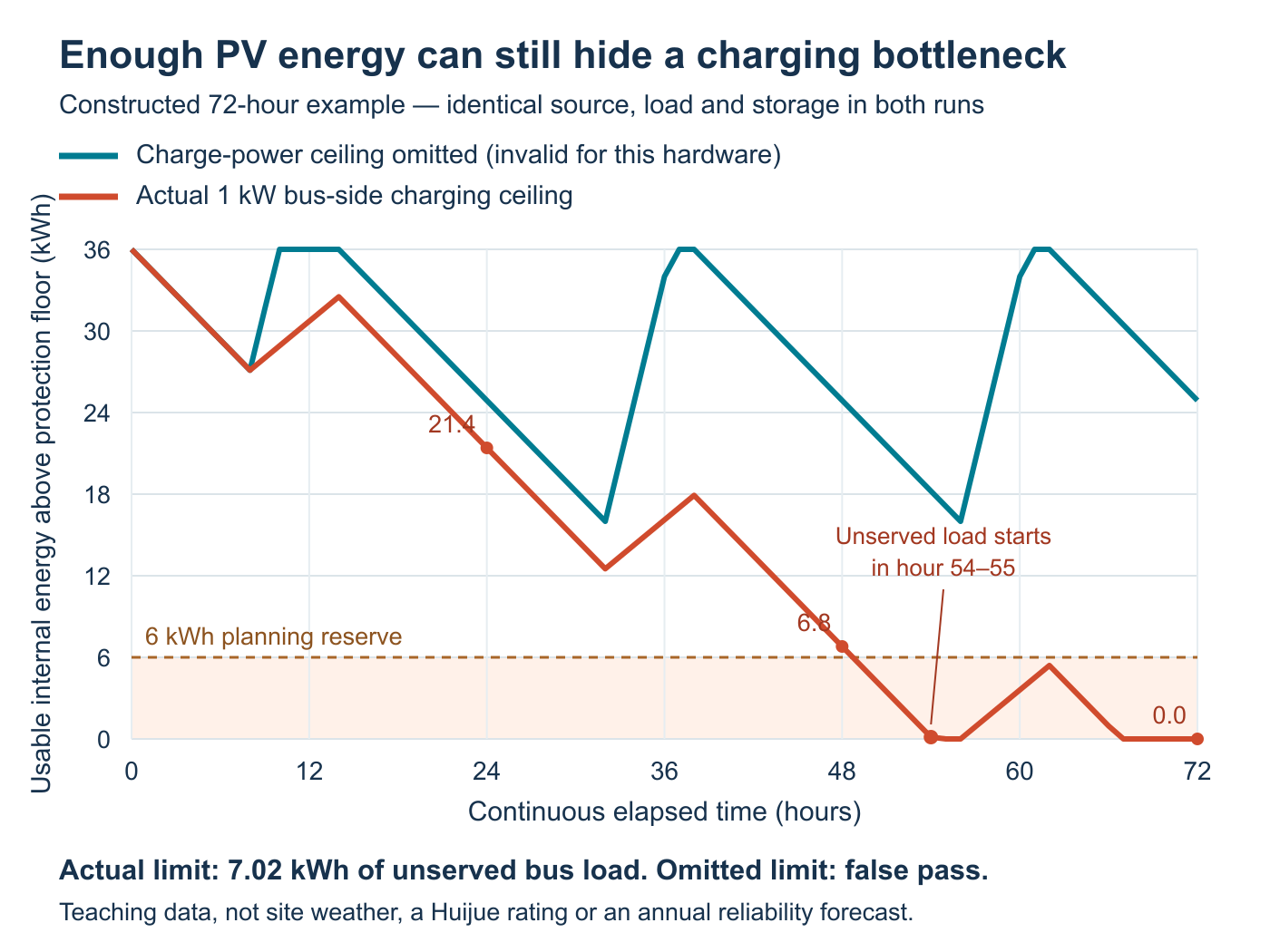
View the calculated energy trace at full size.

With the 1 kW ceiling, day-end internal energy is 21.4 kWh, 6.8 kWh and then zero. The first hourly endpoint below the planning reserve is 01:00 on Day 3. The first interval containing unserved demand is 06:00–07:00 that day; a small amount remains at its start, so 06:00 is not the precise exhaustion instant. Total unserved load over the example is 7.02 kWh.

The model missing the charging ceiling ends every day at approximately 24.89 kWh, never falls below 16 kWh and reports no unserved load. Both cases retain the same capacity, efficiencies, initial energy and chronological inputs. The apparent pass changes because one model allows charging beyond the stipulated physical limit.

What must carry over from one simulated day to the next?

The battery’s ending energy must become the next interval’s starting energy, together with relevant operating state. A calendar boundary cannot restore a full charge. Initial energy also needs an explicit basis: beginning the calculation full does not establish how the site will regain that condition.

Neither model in this example resets at midnight. Adding a reset would introduce a different error and obscure the isolated charging-limit comparison. In a project model, continue the weather and load sequence through nights, low-production periods and recovery. Check whether an initially favourable charge merely delays a shortage.

The 6 kWh battery reserve is a planning criterion, separate from the protection floor. Continuing the example below that criterion makes the shortfall visible; it does not prescribe real battery operation. The actual site’s approved control and backup policy determines the response to an approaching limit.

Which results must be checked before accepting a solar simulation?

Check unserved critical-load energy, the lowest remaining reserve and when those conditions occur, alongside recovery and the limits applied. Then establish which weather, load and equipment assumptions the result covers. Annual generation or a high average battery level cannot substitute for those observations.

The European Commission JRC’s off-grid PVGIS documentation describes chronological production, consumption and battery calculations, including missing-energy and full/empty-battery outputs. Read each metric’s definition before using it: a percentage of days with an empty battery is not automatically a percentage of service downtime.

A proposed telecom site in Kenya, for example, needs its own coordinates, shading, defensible resource series and telecom load profile. The constructed trace above supplies none of that location evidence. Real charging acceptance may also vary with temperature, battery state and converter derating; a fixed ceiling is only the stipulated condition used to isolate this example’s error.

A 72-hour pass would remain limited to those 72 hours and assumptions. Longer resource sequences, adverse operating conditions and growth cases still require review. An hourly energy calculation cannot verify fast load transients, protection coordination or failure response, nor establish annual service availability by itself.

Turn the failed interval into a design decision

Hold reliance on the optimistic result until the model represents the offered charging path. Identify which converter, BMS or operating restriction sets the limit, correct that input and rerun the same sequence. If a proposed equipment change raises the limit, verify the complete affected path before treating the revised trace as achievable.

The corrected result should show what changed and whether the shortage remains. That makes the next discussion concrete: revise the equipment or operating case, extend the analysis, or reject the unsupported pass. A smooth plot alone is not a reason to release the design.